Why I wrote this and who is it intended for?

I realized there’s a gap between understanding how convolution works on 2D images and what the Conv2D operator in most deep learning libraries actually does. And that gap is quite literally an ENTIRE dimension.

If you’ve used CNNs before but can’t fully visualize what your code is doing, or you’ve only seen them in theory during a class, this guide is meant for you.

The difficulty: Visualization

The complexity of figuring out the number of trainable weights in deep learning often comes from the difficulty of visualizing operations in more than three dimensions which is fairly common when working with images.

In fact, that’s a general problem in machine learning. There are many dimensionality reduction techniques, but since we usually work directly with high-dimensional objects, we rarely use them in practice. “High-dimensional objects” might sound pompous, but images which are extremely common already fit into that category.

Images are 3D objects. And it’s not a conspiracy theory.

Let’s say you’re working with an RGB (colored) image. Essentially, it’s three grayscale images stacked on top of each other — one for red, one for green, and one for blue — which makes it a 3-dimensional object.

This might seem unnatural at first because images are perceived as flat — and they are, right? A screen uses clever tricks to fool us into perceiving color. This is what a sub-pixel from a certain brand of TV looks like:

Naturally, we can’t see each sub-pixel individually because they’re tiny by design, and our eyes aggregate the information from the pixel, which is itself made of red, green, and blue light.

So if each pixel is represented by 3 values, and we arrange those pixels on a 2D grid, one faithful way to represent the image without losing any information is to treat it as a 3D block, where the third dimension (depth) holds the RGB channels.

Here’s a small 9x9 image I represented with Spline because I was too lazy to compile Blender. #GentooLife

The gap in your understanding if you’ve been using traditional learning material

Most of us are familiar with this kind of representation:

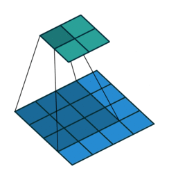
But as I’ve been arguing from the start, we usually work with at least three dimensions. This 2D depiction might make sense for a traditional convolution, but it doesn’t really do the Conv2D operation or you any justice.

A better depiction is this animation from animatedAI:

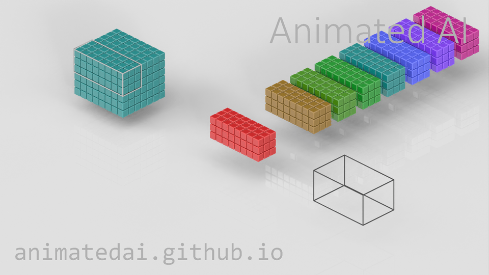
That first block on the top-left can be seen as your input image (or the output from a previous layer). Notice how there are more than three “features” in the depth dimension. This is a more general depiction of an image. Other channels could represent things like transparency, heat, etc.

The filter array in the middle where you see many 3 × 3 × I blocks is a stack of multiple feature maps. Each 3 × 3 × I block is a single filter (or kernel or feature map), spanning the entire depth of the input.

Now let’s connect this to the APIs you’ll actually use. Here’s the PyTorch version:

class torch.nn.Conv2d(in_channels,
out_channels,
kernel_size,
stride=1,
padding=0,
dilation=1,
groups=1,
bias=True,
padding_mode='zeros',
device=None,
dtype=None)

Here’s the tensorflow way

tf.keras.layers.Conv2D(
    filters,
    kernel_size,
    strides=(1, 1),
    padding='valid',
    data_format=None,
    dilation_rate=(1, 1),
    groups=1,
    activation=None,
    use_bias=True,
    ...,
    **kwargs
)

The kernel_size parameter is common, in our animation that’s the “3”. Hence the 3 x 3 in the 3 x 3 x I.

This is how Tensorflow documentation describe the filters:

filters :int, the dimension of the output space (the number of filters in the convolution).

And this is how Pytorch documentation describe the out_channel:

out_channels:int, Number of channels produced by the convolution

The kernel_size parameter is common to both — that’s the “3” in the 3 × 3 × I.

TensorFlow describes filters as:

filters: int, the dimension of the output space (the number of filters in the convolution).

PyTorch describes out_channels as:

out_channels: int, number of channels produced by the convolution.

Once we combine this with the animation, the idea becomes straightforward:

The number of filters/out_channels determines the depth of the resulting image.
The in_channels correspond to the depth of the input, and therefore the depth of each kernel.

Quick recap: Less abstraction, just 3D images, Python, and kindergarten math

So we have a 3D image. We pass it through a Conv2D block in TensorFlow or PyTorch.

Assuming padding, stride, and dilation are left at their defaults, and this is your first trainable layer, it might look something like this:

import tensorflow as tf
from tensorflow.keras import layers, models


target_size = (200, 200)
input_shape = (None, None, 3)

model_a = models.Sequential([
    layers.Input(shape=input_shape),
    layers.Resizing(*target_size),  # force 200x200
    #vvvvvvvvvvvvvvvvvvvvvvvvvvvvvvvvvvvvvvvvvvvv
    layers.Conv2D(filters=16, kernel_size=(1, 1))
    #^^^^^^^^^^^^^^^^^^^^^^^^^^^^^^^^^^^^^^^
])

model_a.summary()

Layer (type)	Output Shape	Parameters
resizing (Resizing)	(None, 200, 200, 3)	0
conv2d (Conv2D)	(None, 200, 200, 16)	64

This might look like a trivial example, since a 1x1 convolution maps each input pixel to an output pixel directly but it’s still very useful for confirming our visual intuition and 1x1 convolution are often used to change the channel count.

Our in_channels was 3 (RGB), and our out_channels / filters was 16. That matches exactly with the animation: input depth → 3, output depth → 16.

Now look at the parameter count: 64. Let’s break it down.

The number of parameters is:

\[ P_c = (\text{kernel\_width} \times \text{kernel\_height} \times \text{in\_channels} + 1) \times \text{out\_channels} \]

The term inside the parentheses represents the parameter count of a single filter:

\[ F_{m_c} = \text{kernel\_width} \times \text{kernel\_height} \times \text{in\_channels} + 1 \]

That +1 accounts for the bias. Same idea as in a multilayer perceptron just extended into 3D. And since we have one filter per output channel, we multiply this by out_channels.

Here: kernel_size = 1, in_channels = 3, out_channels = 16

\[ F_{m_c} = 1 \times 1 \times 3 + 1 = 4 \]

And finally:

\[ P_c = 4 \times 16 = 64 \]

Images are actually 3D objects,reality is a lie,and how to understand the Conv2d layer in CNN

Why I wrote this and who is it intended for?

The difficulty: Visualization

Images are 3D objects. And it’s not a conspiracy theory.

The gap in your understanding if you’ve been using traditional learning material

Quick recap: Less abstraction, just 3D images, Python, and kindergarten math

Further reading / looking