About this post
This is probably the longest post I’ve ever written. Hence, I decided to break it down into several parts. This is the first one.
I’m trying my best to make this post accessible to the maximum number of people, so there are several ways to engage with the content:
If you don’t care much about the theoretical details and you’re just here for the anecdotes and the history, don’t toggle the “theoretical example” callout.
If you have solid fundamentals in statistics and calculus and you’re brave enough, give them a try. If you don’t understand some derivations, blame me for not making it clear not yourself. You got this!
And for the industry experts: I don’t think you’re going to learn much from the overly detailed math sections, but I will gladly take any proof-checker I can get.
I hope you will like it :)
In the beginning was the “artificial neural network”
Sooo, let me kick things off with a rant. I really hate the term Artificial Intelligence, because in practice we’re still far from intelligent programs.
We’re working with advanced statistical machines, but some breakthroughs in the field were indeed bio-inspired. This article will be packed with nerdy references and statistical jokes. Hopefully, you will recognize them as jokes since it’s not my forte.
Anyway, the artificial neural network is one such example of a statistical machine.
You can think of it as a simplistic mathematical representation of a neuron.
A logical calculus of the ideas immanent in nervous activity (1943)
It started with the assumption that a neural network has neurons with binary states. Binary outputs are easy to represent mathematically, so that was a good starting point. The next step was thinking about the neural network as a graph or a network in the mathematical sense.
\[ N_i(t) \in \{0, 1\}, \quad N_i(t) = 1 \text{ (firing)}, \; N_i(t) = 0 \text{ (not firing)}. \]
Each connection \(j \to i\) has weight \(w_{ij}(t) \in \mathbb{Z}\) (excitatory if \(w_{ij} > 0\), inhibitory if \(w_{ij} < 0\)).
Each neuron \(i\) has a threshold \(\theta_i(t)\). Its next state is given by
\[ N_i(t + 1) = H\left(\sum_{j=1}^{n} w_{ij}(t)N_j(t) - \theta_i(t)\right), \]
with
\[ H(x) = \begin{cases} 1, & x \ge 0 \\ 0, & x < 0 \end{cases}. \]
Eventually the definition changed a bit, and after a lot of work, we got the perceptron, thanks to Frank Rosenblatt in 1957.
The astute reader who also happens to be a statistician might notice the resemblance between the formula inside the H and a linear regression equation. That’s because… it is essentially a linear regression.
The \(w_{ij}\) are your usual \(\beta_i\), and \(\theta_i\) is your \(β_0\), the value at the origin.
And the perceptron was… bad. Like, really bad.
The first neural networks were essentially trying to make predictions by fitting every data point on a line and making predictions using this heuristic.
As you can guess, this didn’t go far because people have complex data problems. Or at least they believe they do, and that’s how my fellow data scientists and I stay employed.
Eventually, someone pointed out that this was too naive. One of the most famous overly complicated ways to show that not everything fits on a line is the XOR problem.
| A | B | A XOR B |
|---|---|---|
| 0 | 0 | 0 |
| 0 | 1 | 1 |
| 1 | 0 | 1 |
| 1 | 1 | 0 |
I’m currently too lazy to draw a graph, but looking at the table above and using your imagination, you might realize that the only non-zero points appear at (1,0) and (0,1). That’s a long way to say that a simple line can’t explain a XOR gate.
Now, in 1969, Marvin Minsky and Seymour Papert published a book called… you guessed it… Perceptrons. Book titles were simpler back then.
The book highlighted the limits of perceptrons which you, dear reader, have realized without needing to write an entire mathematics book. But here we are. That’s the price of making history.
This book almost single-handedly stopped neural network research. I’m exaggerating a bit, but it was a big deal. Funding for neural network research became difficult,yet the scientific community kept pushing forward.
At the time, some people knew that using a Multi-Layer Perceptron (MLP) could fix the XOR problem, but nobody knew about backpropagation yet, so progress stalled.
Anecdotally, Rosenblatt predicted that perceptrons would “eventually be able to learn, make decisions, and translate languages”. And actually he was right.
And then we discovered backpropagation ~ 1986
Depending on your background, you might already be familiar with backpropagation. If so, feel free to jump to the next section.
If you’re not, and you just want a basic intuition for what it does and why it was (and still is) a big deal, I’ll try to be concise.
Think of neural networks as function approximators. They have several parameters you can adjust to get the best approximation. (In linear regression, you’re tweaking the value at the origin and the slope to find the line that best matches your data.)
Now, how do you find the parameters that give you the best fit? Backpropagation is one way to do it.
The core idea is that your neural network is a function of both the parameters and the data. For a given data point, backpropagation uses derivatives, notably the chain rule, to determine how to update the parameters to improve the fit.
Several people discovered it at the same time. (Shoutout to Yan Le Cun David E. Rumelhart, Geoffrey E. Hinton & Ronald J. Williams) !
And this discovery reignited the field. We could finally solve the XOR problems and problems that were way more complex. This method is still being used today to train most neural networks.
If you want to know in details how it’s applied to solve the XOR problem with a 2-layer MLP you can look at the hidden section.
The Setup, a 2-Layer MLP
Let’s look at a simple network with one hidden layer. We neglect the bias term here to keep things readable.
- Input: \(x\)
- Hidden Layer: Weights \(W_1\), output \(h\)
- Output Layer: Weights \(W_2\), prediction \(y\)
The forward pass:
Hidden layer: \(z_1 = W_1 x \rightarrow h = f(z_1)\)
Output layer: \(z_2 = W_2 h \rightarrow y = f(z_2)\)
Loss: compute \(L(y, \text{target})\)
The goal: We want the gradients of the loss with respect to both weight matrices, so we can update them during training:
\[ \frac{\partial L}{\partial W_2} \quad \text{and} \quad \frac{\partial L}{\partial W_1} \]
If you have ever taken a physics class, you might have seen a professor treat derivatives like simple fractions. When introducing the chain rule, they casually say:
“See, the \(dy\)’s just cancel out.” \[ \frac{dx}{dy} \cdot \frac{dy}{dz} = \frac{dx}{dz} \]
And to that I will say, do not hate the players, hate the game.
If not fraction, why fraction like ???
This level of understanding is good enough to follow what comes next. And if you are new to this, do not bash yourself if you do not understand everything, writing it out myself was painful and I may have included a typo or two.
Part 1, the output layer (\(W_2\))
We start at the end. This part is the easy one, because the weights \(W_2\) are directly connected to the loss.
Yes, it gets worse, really fast.
The chain rule map
We retrace the path from the loss back to \(W_2\):
\[ L \leftarrow y \leftarrow z_2 \leftarrow W_2 \]
| Derivative component | Expression | Why |
|---|---|---|
| Loss w.r.t prediction | \[ \frac{\partial L}{\partial y} \] | The slope of the loss function, for example MSE or cross entropy. |
| Prediction w.r.t pre-activation | \[ \frac{\partial y}{\partial z_2} = f'(z_2) \] | The derivative of the activation function at the output. |
| Pre-activation w.r.t weights | \[ \frac{\partial z_2}{\partial W_2} \rightarrow h^T \] | If this feels magical, matrix calculus is your friend. |
The derivation
Putting these pieces together:
\[ \frac{\partial L}{\partial W_2} = \frac{\partial L}{\partial z_2} \cdot \left(\frac{\partial z_2}{\partial W_2}\right) = \left[ \frac{\partial L}{\partial y} \cdot \frac{\partial y}{\partial z_2} \right] \cdot \left(\frac{\partial z_2}{\partial W_2}\right) \]
Which simplifies to:
\[ \frac{\partial L}{\partial W_2} = \left[ \frac{\partial L}{\partial y} \cdot f'(z_2) \right] \cdot h^T \]
Let’s give a name to the term in brackets, \(\delta_2\):
\(\delta_2\), the error term for layer 2.
It measures how sensitive the loss is to the pre-activation \(z_2\).
\[ \delta_2 = \frac{\partial L}{\partial z_2} = \frac{\partial L}{\partial y} \odot f'(z_2) \]
Here \(\odot\) denotes element-wise multiplication.
So finally:
\[ \frac{\partial L}{\partial W_2} = \delta_2 \cdot h^T \]
The final stitching
Now we plug everything together to see the full chain in action.
\[ \frac{\partial L}{\partial W_1} = \Bigg[ \bigg( W_2^T \cdot \delta_2 \bigg) \odot f'(z_1) \Bigg] \cdot x^T \]
\[ \frac{\partial L}{\partial W_2} = \delta_2 \cdot h^T \]

And the Recurrent Neural Networks era started
There’s a phenomenon which happens all the time when we speak that I find fascinating, because I worked on speech synthesis last summer, but I was pleasantly surprised to see that I wasn’t alone in this. I’m talking about coarticulation.
Coarticulation is quite simple to explain actually. The way you pronounce something at some point depends on what you said before and what you will say after.
We all do it naturally when we talk, with rap music or slam being among the situations where it’s the most obvious.
Now let’s say that you’re interested in a robot that could rap. And you only had one shot, one moment to make it perform a verse. How would you capture it?
MLPs shortcomings
The difficulty here is that MLPs are not really cut for these kinds of tasks. An MLP processes inputs independently, it has no internal memory(memory is an import notion for this series) of what came before, so the only way to handle sequences is to feed it a fixed-length context window, or to hand-engineer features summarizing the past. If you train an MLP to predict the third sound based on the first two, then that’s all you will get. If you later decide that you need to factor three or four previous sounds, you need a different model, new parameters, and a new training procedure. This makes MLPs brittle for sequential problems, where context length is variable and ordering matters.
Recurrent Neural Networks were introduced precisely to solve this. Instead of treating each input independently, an RNN maintains a hidden state that summarizes past inputs. This hidden state is carried across time steps, which means the model explicitly represents temporal dependencies. The same parameters are reused at every time step, giving the model a consistent way to process each element in the sequence, while keeping the number of parameters manageable. Because of this, RNNs naturally handle variable-length inputs, preserve time order, and can be used in one-to-many, many-to-one, or many-to-many sequence mappings, without requiring fixed-size encodings.
This also makes them suitable for online or streaming tasks like freestyle rapping. Since the model processes data step by step, it can update its predictions as new inputs arrive, instead of needing the entire sequence upfront.
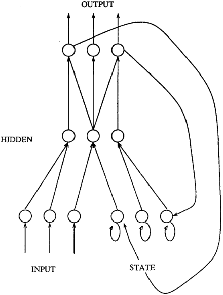
At the time, people were talking about Parallel Distributed Processing, or PDP. It was a broader framework, but Michael I. Jordan presented what we would now call an RNN, with a modern lens, in his PhD thesis.
From there, things picked up quickly. We got Backpropagation Through Time, an adaptation of backpropagation for RNNs, and Rosenblatt’s prediction became true.
For the curious and tenacious, I wrote a similar theoretical explanation of how it works in practice.
The Setup: A Simple 3-Step RNN
Let’s assume an RNN that runs for exactly 3 time steps (\(t=1, 2, 3\)). Our goal is to update the weight matrix \(W_{hh}\) (hidden-to-hidden weights).
The Forward Pass:
At each step, we calculate a “pre-activation” \(z\) and an “activation” \(h\).
Time 1: \(z_1 = W_{hh}h_0 + W_{hx}x_1 \rightarrow h_1 = f(z_1) \rightarrow L_1\)
Time 2: \(z_2 = W_{hh}h_1 + W_{hx}x_2 \rightarrow h_2 = f(z_2) \rightarrow L_2\)
Time 3: \(z_3 = W_{hh}h_2 + W_{hx}x_3 \rightarrow h_3 = f(z_3) \rightarrow L_3\)
The Goal:
We want the derivative of the Total Loss \(L = L_1 + L_2 + L_3\) with respect to the shared weight matrix \(W_{hh}\).
\[ \frac{\partial L}{\partial W_{hh}} = \frac{\partial L}{\partial W_{hh}}\bigg|_{t=1} + \frac{\partial L}{\partial W_{hh}}\bigg|_{t=2} + \frac{\partial L}{\partial W_{hh}}\bigg|_{t=3} \]
Part 1: The End of Time (\(t=3\))
We start our derivation at the very last time step and work backward.
At \(t=3\), the hidden state \(h_3\) has only one job: produce the output loss \(L_3\). There is no \(t=4\), so there are no future consequences for \(h_3\).
The Chain Rule Map
We need to find the derivative of the Loss w.r.t \(W_{hh}\) at this specific step. Let’s map the path: \[ L_3 \leftarrow h_3 \leftarrow z_3 \leftarrow W_{hh} \]
| Derivative Component | Mathematical Expression | Why? |
|---|---|---|
| Loss w.r.t Activation | \[ \frac{\partial L_3}{\partial h_3} \] | How much the loss changes if the hidden state changes. |
| Activation w.r.t Pre-activation | \[ \frac{\partial h_3}{\partial z_3} = f'(z_3) \] | The derivative of our activation function (e.g., tanh). |
| Pre-activation w.r.t Weights | \[ \frac{\partial z_3}{\partial W_{hh}} = h_2 \] | Looking at \(z_3 = W_{hh}h_2 + \dots\), the coefficient of \(W_{hh}\) is the previous state \(h_2\). |
The Derivation
Combining these terms (remembering to transpose matrices to match dimensions):
\[ \text{Gradient}_3 = \left[ \frac{\partial L_3}{\partial h_3} \cdot f'(z_3) \right] \cdot h_2^T \]
Part 2: The Middle Child (\(t=2\))
Now things get interesting. We move back to \(t=2\).
The hidden state \(h_2\) is responsible for two things:
The Present: It helps generate \(L_2\).
The Future: It is used to calculate \(h_3\), which creates \(L_3\).
Therefore, the gradient of the Loss with respect to \(h_2\) is not just about \(L_2\). It is the sum of the immediate loss and the Gradient from the Future.
The Chain Rule Map (Backpropagating from \(t=3\))
To find the “Gradient from the Future,” we look at how \(h_2\) influences \(L_3\).
\[ L_3 \leftarrow h_3 \leftarrow z_3 \leftarrow h_2 \]
| Derivative Component | Expression | Why? |
|---|---|---|
| Future Loss w.r.t Future Activation | \[ \frac{\partial L_3}{\partial h_3} \] | Calculated in Part 1. |
| Future Activation w.r.t Future Z | \[ \frac{\partial h_3}{\partial z_3} = f'(z_3) \] | Calculated in Part 1. |
| Future Z w.r.t Current Activation | \[ \frac{\partial z_3}{\partial h_2} = W_{hh} \] | Looking at \(z_3 = W_{hh}h_2 + \dots\), the derivative of \(z_3\) w.r.t \(h_2\) is the weight matrix itself. |
Step 2.1: The Cumulative Gradient at \(h_2\)
Let’s define a specific term for the total sensitivity of the network to changes in \(h_2\). This includes the loss at step 2, and the loss at step 3.
\[ \frac{\partial L_{\text{total}}}{\partial h_2} = \underbrace{\frac{\partial L_2}{\partial h_2}}_{\text{Present}} + \underbrace{ \left[ \frac{\partial L_3}{\partial h_3} \cdot f'(z_3) \right] W_{hh}^T }_{\text{Future (Backpropped from } t=3 \text{)}} \]
Step 2.2: Descent to \(W_{hh}\)
Now that we have the total gradient at \(h_2\), we continue down the chain to \(W_{hh}\) (via \(z_2\)). \[ \text{Gradient at } h_2 \rightarrow z_2 \rightarrow W_{hh} \]
\[ \text{Gradient}_2 = \left[ \underbrace{\left( \frac{\partial L_2}{\partial h_2} + \left[ \frac{\partial L_3}{\partial h_3} \cdot f'(z_3) \right] W_{hh}^T \right)}_{\text{Cumulative Gradient at } h_2} \cdot f'(z_2) \right] \cdot h_1^T \]
Part 3: The Deepest Recursion (\(t=1\))
We finally arrive at the start. \(h_1\) is the parent of everything. It creates \(L_1\). It creates \(h_2\) (which creates \(L_2\)). It indirectly creates \(h_3\) (which creates \(L_3\)).
The Chain Rule Map (Backpropagating from \(t=2\))
We need to pull the “Cumulative Gradient at \(h_2\)” (which we just calculated) back one more step to \(h_1\).
| Derivative Component | Expression | Why? |
|---|---|---|
| Cumulative Gradient at \(h_2\) | \[ \frac{\partial (L_2+L_3)}{\partial h_2} \] | Calculated in Part 2. |
| Next Z w.r.t Current Activation | \[ \frac{\partial z_2}{\partial h_1} = W_{hh} \] | Linking step 2 back to step 1. |
Step 3.1: The Cumulative Gradient at \(h_1\)
This is the sum of the direct loss (\(L_1\)) and the entire stream of errors flowing back from the future (\(t=2, 3\)).
To get the future error to \(h_1\), we take the Total Gradient at \(h_2\), pass it through the activation derivative \(f'(z_2)\), and then through the transition matrix \(W_{hh}^T\).
\[ \frac{\partial L_{\text{total}}}{\partial h_1} = \frac{\partial L_1}{\partial h_1} + \underbrace{ \left[ \text{Cumulative Gradient at } h_2 \cdot f'(z_2) \right] W_{hh}^T }_{\text{All Future Errors}} \]
Step 3.2: The Full Expansion
If we expand the term “Cumulative Gradient at \(h_2\)” with the equation from Part 2, we get a nested structure.
\[ \frac{\partial L_{\text{total}}}{\partial h_1} = \frac{\partial L_1}{\partial h_1} + \left[ \left( \frac{\partial L_2}{\partial h_2} + \left[ \frac{\partial L_3}{\partial h_3} \cdot f'(z_3) \right] W_{hh}^T \right) \cdot f'(z_2) \right] W_{hh}^T \]
Step 3.3: Descent to \(W_{hh}\)
Finally, we calculate the weight update for this time step by passing through \(z_1\).
\[ \text{Gradient}_1 = \left[ \frac{\partial L_{\text{total}}}{\partial h_1} \cdot f'(z_1) \right] \cdot h_0^T \]
The Final Result
The total gradient for \(W_{hh}\) is the sum of the gradients calculated at each time step. \[ \frac{\partial L}{\partial W_{hh}} = \text{Gradient}_1 + \text{Gradient}_2 + \text{Gradient}_3 \]
If we substitute the expanded versions we just derived, we can see the full “Backpropagation Through Time” equation.
\[ \frac{\partial L}{\partial W_{hh}} = \]
\[ \underbrace{ \Bigg[ \bigg( \frac{\partial L_1}{\partial h_1} + \underbrace{ \bigg[ \underbrace{ \Big( \frac{\partial L_2}{\partial h_2} + \underbrace{ \Big[ \frac{\partial L_3}{\partial h_3} \cdot f'(z_3) \Big] W_{hh}^T }_{\text{Signal from } L_3 \to h_2} \Big) }_{\text{Total Gradient at } h_2} \cdot f'(z_2) \bigg] W_{hh}^T }_{\text{Signal from } L_2, L_3 \to h_1} \bigg) \cdot f'(z_1) \Bigg] h_0^T }_{\text{Gradient 1 (Contribution from } t=1)} \]
\[ + \]
\[ \underbrace{ \Bigg[ \bigg( \frac{\partial L_2}{\partial h_2} + \underbrace{ \Big[ \frac{\partial L_3}{\partial h_3} \cdot f'(z_3) \Big] W_{hh}^T }_{\text{Signal from } L_3 \to h_2} \bigg) \cdot f'(z_2) \Bigg] h_1^T }_{\text{Gradient 2 (Contribution from } t=2)} \]
\[ + \]
\[
\underbrace{ \Bigg[ \frac{\partial L_3}{\partial h_3} \cdot f'(z_3) \Bigg] h_2^T }_{\text{Gradient 3 (Contribution from } t=3)}
\] 
Why Going Through ALL OF THIS Was Worth It: The Vanishing Gradient
By writing out the full chain rule for Gradient 1, we can clearly see the repeated multiplication of \(W_{hh}\).
To get the error signal from \(L_3\) all the way back to the update at \(t=1\), we had to multiply by \(W_{hh}\) twice (once to go \(3 \to 2\), and once to go \(2 \to 1\)).
If we had 100 time steps, we would see \(W_{hh}\) multiplied by itself 99 times.
If \(W_{hh}\) has values small than 1, \(0.9^{99} \approx 0.00003\). The signal vanishes.
If \(W_{hh}\) has values larger than 1, \(1.1^{99} \approx 12527\). The signal explodes.
And that is why, historically, RNNs were so hard to train until LSTMs and GRUs came along to “protect” that gradient flow!
That’s it for now ! In the next part I will cover RNN’s more extensively but in the meantime, here’s a reading/watching list if you want to learn more about them.